Open Quantum Systems

Dynamics of Open Quantum Systems

In practical settings, the many-body quantum systems can not be truly isolated, underscoring the importance of open many-body quantum systems. A prominent example of an open quantum system is a quantum computer where qubits interact with each other and their surrounding environment. Studying open quantum systems brings its own set of challenges, especially in modeling the interaction between the system and environment. The study of open quantum systems is somewhat limited to the weak coupling between the system and the environment (Markov approximation). Recent developments utilizing process tensors have made handling the non-Markovian environment for studying open quantum systems accessible.I am currently working on the non-markovian dynamics of open quantum systems for my Master's thesis.

I started with the unbiased spin-boson model to investigate the effects of dissipation on a quantum system. This model describes a quantum particle in a dissipative bath of the harmonic oscillator. The Hamiltonian of this model is described below $\begin{equation*} H = \Omega S_x + \mathop {\sum}\limits_i S_z\left( {g_ia_i + g_i^ \ast a_i^\dagger } \right) + \omega _ia_i^\dagger a_i \end{equation*}$ where $S_x$ and $S_z$ are spin operators, $a_i$ $(a_i ^\dagger)$ are annihilation (creation) operators, $w_i$ is the $i$ th frequency mode of the bath, and $g_i$ , the coupling strength between the system and the bath. The behavior of the bath is characterized by the spectral density function

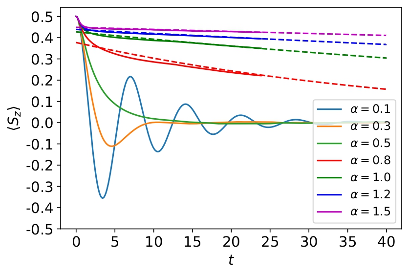
Fig. 1 : The dynamics of the spin-1/2 system captured at K = 200 for the different values of $\alpha$ indicated. The dotted lines show the exponential fits to the data above $\alpha = 0.5$ .

$\begin{equation*} J(\omega ) = \mathop {\sum}\limits_i \left| {g_i} \right|^2\delta \left( {\omega - \omega _i} \right) \end{equation*}$

For ohmic spectral density $J(\omega ) = 2\alpha \omega \,{\mathrm{exp}}( - \omega /\omega _{\mathrm{c}})$ , this model shows a quantum phase transition at critical value of the system-environment coupling $\alpha=\alpha _c$ . The time-evolving matrix product operator (TEMPO) algorithm has been employed for the calculation, which exploits the augmented density tensors (ADT) to capture the system's history over a finite bath memory time $\tau_c$ . Figure 1 shows the evolution of $\langle S_z(t) \rangle$ , with an initial condition $\langle S_z(t=0) \rangle = + \frac{1}{2}$ and with no excitations in the environment. Before reaching the localized phase, there is a crossover at $\alpha \cong 0.5$ from coherent decaying oscillation to incoherent decay. For $\alpha > 0.5$ , $\langle S_z \rangle$ decays to zero asymptotically as $\langle S_z(t) \rangle \propto \exp(-\gamma t)$ as shown in figure 1.

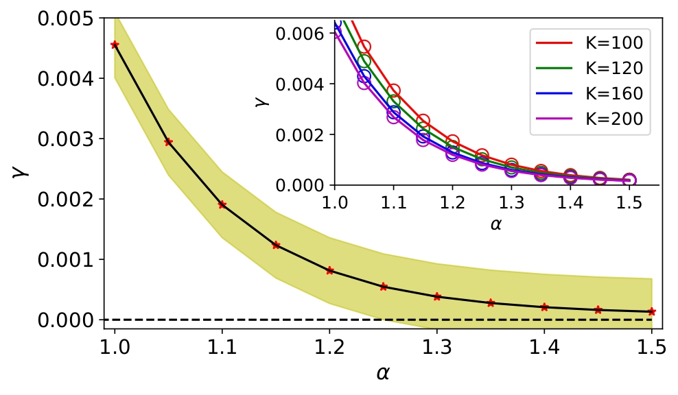
Fig. 2 : Shows the extrapolated decay rate $\gamma$ which crosses zero at around $\alpha \cong 1.25$ .The inset shows the dependence of the decay rate $\gamma$ of the exponential fit on 1/K \& is utilized to extract the value of $\gamma$ when $K \rightarrow \infty$ .

However, at large $\alpha$ , $\langle S_z \rangle$ approaches a non-zero value asymptotically when the system localizes. The decay rate $\gamma$ crosses zero at around $\alpha _c \cong 1.25$ with a $90\%$ confidence interval as depicted in figure 2 where the inset shows the dependence of the decay rate $\gamma$ with memory cutoff $\tau _c \rightarrow K \Delta$ . The system transitions from the delocalized phase to a localized phase at around $\alpha _c \cong 1.25$ , consistent with the known result.